
Chapter 4: Display
|
4-11: Waveform Windows | |
The waveform window is able to display simulation output and cross-probe it to the layout or schematic. This simulation output can come from external simulators (such as Spice and Verilog) or from built-in simulators (such as ALS and IRSIM). When displaying the results of external simulators, it reads the simulation output and shows it. When internal simulators are displayed, you have the additional capability of changing the stimuli.
The waveform window looks like the picture below. Note that there is a side bar with a cell explorer in the window, just like in all windows, but the explorer has a "SIGNALS" section that lists the signals found in the simulation (and optionally a "SWEEPS" section if swept data was found). When reading HSpice data, the signals and sweeps sections may be further qualified by analysis, for example "TRANS SIGNALS", "DC SIGNALS", etc.
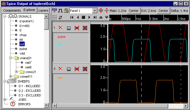
The waveform window contains a set of panels, each with one or more signals. There is a "current panel" which is identified with a thicker vertical axis (the top panel in the above picture). In a panel, signal names are shown on the left, and their waveform on the right. Above the signal names in each panel are a number of controls:
You can create a new panel, with no signals in it, by clicking on the button in the upper-left of the waveform window
( ) or by using the Create New Waveform Panel command
(in menu Window / Waveform Window).
) or by using the Create New Waveform Panel command
(in menu Window / Waveform Window).
| When viewing digital simulation output (such as Verilog) waveforms can be busses. Busses are collections of single signals that display integer values (for example, "path[0:31]"). To see the individual signal that make up a bus, double-click the bus signal (and double-click it again to remove the individual signals). | 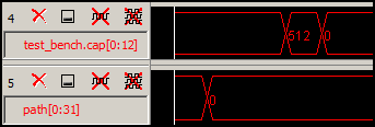 |
You can see new signals by double-clicking on the name in the "SIGNALS" area. For digital simulations, a new panel will be created for that signal; for analog simulations, the signal will be added to the current panel. You can also add signals to a panel by dragging the text onto the panel. Signal names in panels can be renamed by double-clicking on their text (this does not rename the actual signal in Electric: it merely assigns an "alias" name to the signal in the waveform window, which is useful for documentation).
If the layout or schematics cell that produced the simulation is being displayed in another window, and a network is selected in that window, then that network can be added to the waveform window with the Add to Waveform in New Panel command (in menu Edit / Selection). The command Add to Waveform in Current Panel overlays the signal on top of others in the currently selected waveform panel.
You can rearrange the order of the waveform panels by clicking on their panel-number and dragging the panel to a new location. You can move signals from one panel to another by dragging their names to their desired panel. If you use shift-click to drag signals, they are copied to the new panel.
You can change the color of a signal by right-clicking on its name and choosing a different color. When viewing digital waveforms, the color can also vary with the strength of the signal. To enable such a display, check "Multistate display" in the Simulators Preferences (in menu File / Preferences..., "Tools" section, "Simulators" tab). To control the actual colors used in multistate display, use the Layers Preferences (in menu File / Preferences..., "Display" section, "Layers" tab) and set the colors for "WAVEFORM: OFF STRENGTH", "WAVEFORM: NODE (WEAK) STRENGTH", "WAVEFORM: GATE STRENGTH", and "WAVEFORM: POWER STRENGTH" (see Section 4-6-2).
The order of signals in the waveform window is saved so that subsequent simulations will show the same signals. You can also save the configuration of the waveform window with the Save Waveform Window Configuration to Disk... command (in menu Window / Waveform Window) and you can restore the configuration with the Restore Waveform Window Configuration from Disk... command.
The Export Simulation Data... command (in menu Window / Waveform Window) writes a tab-separated file with all simulation data (names and values). The Export Simulation Data As CSV... command writes a comma-separated file with all simulation data. These commands are useful for doing spreadsheet analysis of the data.
If the simulation had sweeps, those values are shown in the cell explorer in a separate "SWEEPS" area. You can double-click on a sweep to toggle its visibility, or right-click on a sweep and choose to include or exclude it from the display. Right-clicking on the "SWEEPS" icon lets you include or exclude all of them.
A single sweep can be highlighted to distinguish it on the display. Right-click on that sweep and choose "Highlight". To remove all highlighting, right-click on the "SWEEPS" icon and choose "Remove Highlighting".
Two vertical cursors appear in the window, called "main" and "extension" (the extension cursor is dotted). Their time values and their difference are shown at the top of the window. You can click over the cursors and drag them to different time locations. You can also use the "Center" buttons to bring these cursors to the center of the display.
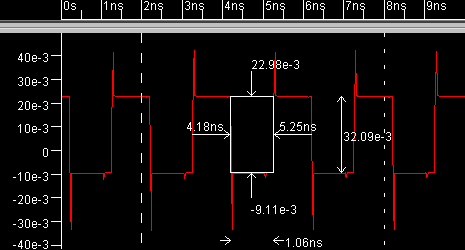 | Another way to measure in the waveform window is to use the "measure" tool (see Section 4-7-4). This tool lets you drag a rectangle, and it shows the left/right time with difference as well as the top/bottom values with difference. The tool snaps to data points so it is easy to get precise measurements. |
The time range in the simulation window can be controlled with the appropriate Window menu commands. Use Zoom Out and Zoom In to scale the time axis by a factor of two. Use Focus on Highlighted (in menu Window / Special Zoom) to display the range between the main and extension cursors.
 | Besides controlling time with menu commands, you can also use the Pan and Zoom tools of the toolbar. |  |
The pan tool lets you smoothly shift time when you click and drag. In the zoom tool, you zoom into an area by clicking and dragging out that area. To zoom out, shift-click in the center of the desired area. You can also adjust time by clicking-and-dragging in the time axis at the top.
| Both the horizontal and vertical axis are drawn linearly. Either axis can be changed to a logarithmic scale by right-clicking on the ruler and choosing "Logarithmic" (use "Linear" to restore the scale). | 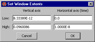 |
You can control the horizontal and vertical range precisely by double-clicking in the vertical scale area. The dialog lets you type exact values into the ranges, and also allows control of log vs. linear as well as scale in the vertical axis. Scale is only allowed for linear plots and only affects the tick marks, not the values.
The different panels in the waveform window are locked in time: they all show the same range of time,
as shown at the top of the waveform window.
If you click on the "time lock" button at the top of the waveform window
(looks like a lock with the time on it:  )
or use the Toggle Horizontal Panel Lock command,
then time is unlocked, and each panel has its own time scale.
Now individual panels can show a different range of time than the rest.
)
or use the Toggle Horizontal Panel Lock command,
then time is unlocked, and each panel has its own time scale.
Now individual panels can show a different range of time than the rest.
A set of VCR buttons is available to animate the main time cursor. The play rate can be controlled by the up-arrow and down-arrow buttons to the right of the VCR controls. These buttons make the playback run faster or slower. As the time cursor sweeps across the waveform window, the original circuit can be seen to change levels. These VCR controls are also available by using the Rewind Main X Axis Cursor to Start, Play Main X Axis Cursor Backwards, Stop Moving Main X Axis Cursor, Play Main X Axis Cursor, Move Main X Axis Cursor to End, Move Main X Axis Cursor Faster, and Move Main X Axis Cursor Slower commands.
These window functions apply to the simulation window:
You can select a signal by selecting either its name or the actual waveform. When you select a signal, and the equivalent schematic or layout is being displayed, Electric does crossprobing and shows the selected network in the schematic/layout. Similarly, when a network in the original schematic or layout is selected, the equivalent waveform is highlighted.
Another feature of crossprobing is the ability to show the electrical state of the network in the original schematic or layout cell (this happens only for digital waveforms). Electric not only highlights the network in the original circuit, but it shows wires with different colors depending on their state (high/low/X/Z) at the current time. If you connect Simulation Probe nodes to any part of the circuit, those nodes light up with the appropriate color instead, which allows better visualization of activity patterns (see Section 7-6-3). You can control the colors used in crossprobing by using the Layers Preferences (in menu File / Preferences..., "Display" section, "Layers" tab) and setting the colors for "WAVEFORM: CROSSPROBE LOW", "WAVEFORM: CROSSPROBE HIGH", "WAVEFORM: CROSSPROBE UNDEFINED", and "WAVEFORM: CROSSPROBE FLOATING" (see Section 4-6-2).
If a Spice deck was generated from the schematic, then crossprobing its simulation results to layout may not work properly. This can be fixed with the Run NCC for Schematic Cross-Probing command (in menu Tools / NCC, see Section 9-7-2).
The horizontal axis does not have to represent time. Any signal can be used in the horizontal axis, simply by dragging that signal onto the horizontal ruler. To restore the horizontal axis to show time, right-click on it and choose "Make the X axis show Time".
When the waveform window displays the output of built-in simulators, you can set stimuli on the signals to affect the simulation. Each stimulus that you set is marked with a large red box at the time of the stimulus. You can select the stimuli by clicking on the red box. A selected stimulus has a green box in it.
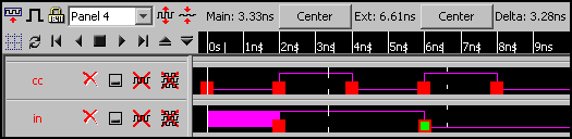
To set stimuli, select either a waveform or the equivalent network in the original schematic or layout. Once selected, use the Set Signal High at Main Time (in menu Tools / Simulation (Built-in)) to make that signal go to "high" at the time indicated by the Main cursor. Use Set Signal Low at Main Time to set the selected signal "low", and use Set Signal Undefined at Main Time to set the selected signal "undefined" (X). Use the Get Information about Selected Signals command to show stimuli and other information on the selected signals.
To remove the selected stimulus, use the Clear Selected Stimuli command. To remove all stimuli on a the selected waveforms, use Clear All Stimuli on Selected Signals. To remove all stimuli in the simulation, use Clear All Stimuli.
| Besides simple test vectors, the ALS simulator can also set clock patterns on the currently selected signal by using the Set Clock on Selected Signal... command. There are two ways to specify a clock: by frequency (in cycles per second) or period (in seconds). | 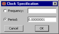 |
Note that the clock cycles infinitely, but Electric generates simulation events to fill only the current waveform window. If you want more clock events generated, zoom-out the waveform window before issuing the clock command.
Once a set of stimuli has been established, you can save it to disk with the Save Stimuli to Disk... command. These stimuli can be restored later with the Restore Stimuli from Disk... command. Each built-in simulator has its own format for saving stimuli.
The Simulators Preferences (in menu File / Preferences..., "Tools" section, "Simulators" tab), offers some controls for built-in simulators.
At the top of the waveform window, above the signal names, are many useful controls. Those relating to time have already been discussed. Here are the remaining buttons:
 Rereads the simulation output file and updates the display.
If the simulation has been re-run, and the output file is different, then this button shows the new data.
This function is also available with the Refresh Simulation Data command
(in menu Window / Waveform Window).
Rereads the simulation output file and updates the display.
If the simulation has been re-run, and the output file is different, then this button shows the new data.
This function is also available with the Refresh Simulation Data command
(in menu Window / Waveform Window).
 Controls the display of dots on the vertices of the waveforms.
The button toggles between three states:
(1) showing lines only, (2) showing lines and dots, and (3) showing dots only.
This is only available for analog waveforms: digital signals are always drawn with lines.
These functions are also available with the Show Points and Lines, Show Lines, and Show Points commands
(in menu Window / Waveform Window).
Controls the display of dots on the vertices of the waveforms.
The button toggles between three states:
(1) showing lines only, (2) showing lines and dots, and (3) showing dots only.
This is only available for analog waveforms: digital signals are always drawn with lines.
These functions are also available with the Show Points and Lines, Show Lines, and Show Points commands
(in menu Window / Waveform Window).
 Displays a grid in the waveform panels.
The button toggles between showing and not-showing the grid.
This function is also available with the Toggle Grid Points command
(in menu Window / Waveform Window).
Displays a grid in the waveform panels.
The button toggles between showing and not-showing the grid.
This function is also available with the Toggle Grid Points command
(in menu Window / Waveform Window).
 These buttons, which show a waveform being stretched or squeezed,
cause the minimum panel size to change.
These functions are also available with the Increase Minimum Panel Height and Decrease Minimum Panel Height commands
(in menu Window / Waveform Window).
By shrinking the panel size, more of them can fit in the window without having to use a slider to access them.
Also, the panels can be resized individually by dragging any of the dividers.
These buttons, which show a waveform being stretched or squeezed,
cause the minimum panel size to change.
These functions are also available with the Increase Minimum Panel Height and Decrease Minimum Panel Height commands
(in menu Window / Waveform Window).
By shrinking the panel size, more of them can fit in the window without having to use a slider to access them.
Also, the panels can be resized individually by dragging any of the dividers.Plotting can be done with special commands in the Window / Waveform Window submenu (see Section 4-8 for more on printing).
An analog signal can be converted to digital with the command Generate Digital Signal from Analog Signal (0.5v threshold) (in menu Window / Waveform Window).
 |
Previous |  |
Table of Contents | Next |  |